All published articles of this journal are available on ScienceDirect.

From Euro III to Clean Buses: Real-world Emissions and Decarbonization Pathways for an Ecuadorian BRT System
Authors Info & Affiliations
Abstract
Introduction
Many large cities, particularly in Latin America, have adopted Bus Rapid Transit (BRT) systems to reduce emissions from individual road transport, yet their impacts on air quality are rarely evaluated. This study aims to estimate fuel consumption and emissions from the BRT fleet in Guayaquil and to explore several decarbonization scenarios.
Methods
The study applies macroscale Tier 1, Tier 2, and Tier 3 methodologies from the European Environment Agency to estimate fuel consumption and emissions of the Guayaquil BRT fleet. Several “what if” decarbonization scenarios are assessed, including upgrading emission-control technologies, switching to low-sulfur fuels and higher biodiesel blends, and incorporating air-conditioning systems. The analysis also accounts for refrigerant leakage and key upstream CO2 emissions from fuel desulfurization and biodiesel production.
Results
The results reveal substantial uncertainty in pollutant inventories. For example, NOX emissions range from 433 to 724 tons per year, depending on the applied methodology. Current palm-oil biodiesel output (16,259 tons per year) is sufficient to supply the Guayaquil BRT fleet without requiring additional land.
Discussion
Although the local biodiesel supply can support the Guayaquil BRT system, extending this bioenergy BRT strategy nationwide would likely generate significant upstream environmental pressures. The findings also highlight variability across emission estimation methods.
Conclusion
The study shows that while the Guayaquil BRT system can be supplied with existing biodiesel production and evaluated through established emission methodologies, scaling such strategies requires careful consideration of upstream environmental impacts and methodological uncertainty.
1. INTRODUCTION
Most Latin American cities face rapid motorization and a growing demand for public transport, with Bus Rapid Transit (BRT) emerging as a key solution for mobility and environmental concerns [1–3]. Given that road transport is a major contributor to urban air pollution and greenhouse gas emissions [4, 5], the accurate quantification of emissions from public transport fleets is critical for designing effective mitigation strategies. Regulatory standards, such as Euro and U.S. limits, provide a framework, but their relevance depends on how vehicles behave in service under conditions very different from those of laboratory testing [6–8].
However, a clear research gap remains in capturing fleet emissions under realistic operating conditions in BRT systems, particularly in Latin American cities. Real-world driving conditions, including variable speeds, idling, acceleration, passenger load, road slope, and air-conditioning use, strongly influence emissions [9–11]. Field studies have shown that nitrogen oxides (NOx) and ammonia (NH3) emissions from buses equipped with aftertreatment systems often diverge significantly from type-approval values [12–15]. Such discrepancies create substantial uncertainty in emissions inventories that cannot be fully resolved by model refinement alone. Instead, integrating real-world measurements with simulation approaches is essential for reducing uncertainty and informing local transport and air quality policies [16, 17].
The need for reliable data has accelerated the interest in complementary monitoring tools. Dense networks of calibrated low-cost sensors, coupled with targeted on-vehicle sampling campaigns, provide the spatial and temporal resolution necessary to assess fleet-scale interventions at a lower cost than traditional stations [18]. Such hybrid approaches allow for the validation of “what-if” scenarios, such as the introduction of low-sulfur fuels, biofuel blends, or retrofitted aftertreatment systems, bridging the gap between modeled expectations and observed urban realities [19]. In addition to driving conditions, additional factors further complicate the emission outcomes. Selective Catalytic Reduction (SCR) systems effectively reduce NOx emissions but may generate ammonia slip [20, 21]. Biodiesel use has been promoted as a decarbonization strategy; however, its influence on regulated pollutants in heavy-duty fleets remains uncertain and often relies on outdated correlations [22–24]. Similarly, air-conditioning operations contribute to both direct refrigerant leaks with high global warming potential and increased fuel consumption from the compressor load [25–27]. These overlapping effects highlight the complexity of predicting fleet emissions and the importance of context-specific evidence before large-scale deployment of new technologies or fuels.
Against this background, the main objective of this study is to simulate the influence of real-world driving conditions on emissions from an Ecuadorian BRT fleet using macroscale regional Tier 1, 2, and 3 inventory methodologies, while explicitly accounting for uncertainty and technology–fuel scenarios. “What-if” simulations are conducted to assess how emissions would change if the current buses adopt different emission-control technologies, switch to low-sulfur fuels, incorporate higher shares of biofuels, and increasingly operate with air-conditioning systems in the coming years [15]. The analysis also quantifies CO2 emissions associated with refrigerant leakage from A/C systems and additional upstream CO2 from desulfurization and biodiesel production plants.
This study contributes by (i) providing a systematic comparison of tier-based emission inventory methods for a Latin American BRT fleet, (ii) delivering an integrated assessment of operational and selected upstream impacts of alternative decarbonization pathways involving fuels, technologies, and A/C use, and (iii) generating evidence that can inform future interventions in urban bus fleets under realistic conditions, with implications for local policy design and broader sustainable transport strategies [28]. The remainder of this paper is organized as follows: Section 2 describes the materials and methods used in this study, including the characterization of the case study and the proposed “what-if” scenarios. Section 3 presents the results, and Section 4 concludes the paper.
2. MATERIALS AND METHODS
2.1. Data Inputs and Emissions Estimations
Emissions from combustion can be estimated based on the mass balance of species present in the fuel and pollutants using Tier 1, 2, or 3 methodologies [29, 30]. Tier methodologies refer to a system, commonly established by the Intergovernmental Panel on Climate Change (IPCC), that uses tiered approaches to estimate greenhouse gas emissions with three levels of increasing complexity and accuracy.
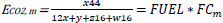
Fleet CO2 and SO2 emissions as mobile combustion sources are directly obtained from the mass combustion balance. For a generic fuel m, a hydrocarbon CxHyOzSw, the complete and non-dissociative combustion chemical reaction is shown in Eq. (1):
CXHᵧOzSw + n(O2 + 3.76N2) → xCO2 + (y/2)H2O + 0.79·nN2 + wSO2 (1)
Therefore, the mass balances for carbon and sulfur are given by the following relationships Eqs. (2 and 3):
 (2)
(2)
 (3)
(3)
Where,
FUEL = 3.14 kg CO2 per kg of fuel (for m = diesel fuel).
kS,m = weight-related sulfur content in fuel of type m (g/g fuel),
FCm = fuel consumption of fuel m (g).
Secondary CO2 emissions are those formed by a process that does not directly involve fuel combustion, such as lube oil leakage and combustion, Air Conditioning (A/C) system leakage, and Selective Catalytic Reduction (SCR) chemical reactions.
The lube oil leaks into the combustion chamber, and the oil film is exposed to combustion and burns along with the fuel. For Tier 1, the mean value was 2.54 gCO2/kg fuel (Euro 4 1.99; uncontrolled 3.32). For Tier 2, a value of 0.486 g/km was assumed. For Tier 3, a leakage of 8.5 kg/10.000 km (for old bus) or 0.85 kg/10.000 km (for new bus) of CH2.08 is assumed, equivalent to 44/(12+2.08) kgCO2/kglube combustion carbon mass balance, or 0.003 g/km (3.12*8.5) and 0.00003 g/km.
Air Conditioning systems (A/C) based on refrigerant fluids with a certain global warming potential could also contribute to secondary CO2 emissions through refrigerant leakage. Generally, mobile A/C systems assembled on cars, trucks, and trains use R134a as the refrigerant of choice. Typically, for a bus, the A/C has 32 kW, weighs 175 kg, and uses 10 kg of refrigerant [26, 31]. A 10.7% fluid leakage accounted for all leakage events from usage. The initial charge depends on the size of the container in kilograms; for the Metrovia system, we assumed a container of 10 kg of R134a refrigerant was used as the initial charge. The carbon dioxide emissions produced by refrigerant fluid leakage were included in this study. The leaks were estimated by multiplying the leakage amount in kg by the Global Warming Potential (GWP) of the refrigerant used Eq. (4):
Refrigerant fluid container (kg) × GWP
As refrigerant gases contribute to global warming potential, mobile A/C systems have started using refrigerant gases with a GWP of less than or equal to 150. Therefore, a future scenario using an R1234yf refrigerant with a GWP of 4 [32–34], which provides lower direct GHG emissions than R134a systems (GWP = 1430; 100 years, [34]), was proposed.
Additionally, nitrogen oxide (NOx) reduction exhaust systems, best known as Selective Catalytic Reduction (SCR) systems, operate with urea injection at the engine exhaust [14, 35]. These aftertreatment devices use an aqueous urea solution as a reducing agent. When urea (NH2)2CO is injected upstream of a hydrolysis catalyst in the exhaust line, the following reaction occurs Eq. (5):
Ammonia is formed in this reaction, which reacts with nitrogen oxides to reduce them to nitrogen. While urea is consumed, it liberates some CO2, which is independent of the CO2 produced by the combustion of the fuel. It is regulated and reported that urea should be in an aqueous solution at a concentration of 32.5% to provide the lowest freezing point and a density of 1.09 g/cm3 [36–40]. If urea solution sales are known, the total CO2 emissions in kilograms produced by urea can be calculated using Eq. (6):
The coefficient 0.26 (kg CO2/lt urea solution) considers the density of the urea solution, molecular masses of CO2 and urea, and urea content in the solution. Usually, urea consumption is 5-7% of fuel consumption at the Euro V level and 3-4% at the Euro VI level.
For pollutant emissions, CO, NMVOC, NOx, PM2.5, and NH3, there are several possible approaches, even at the macroscale level [41], considering the European Environment Agency (EEA) road transport methodology [42].
2.1.1. A/C Usage Effect on Fuel Consumption and Emissions
Among auxiliary systems, the air conditioning systems in vehicles are the major contributors to the gap between laboratory test emissions and real-world emissions. Air conditioning systems could represent an increase of 11 – 14% in fuel consumption [9].
Extra fuel consumption and CO2 emissions of a mobile air-conditioning system for a given environment Temperature (T) and relative Humidity (H) can be calculated for passenger cars using the Tier 3 approach. For buses, there is no methodology, and the objective is to update the light-duty data to heavy-duty buses using a Correction Factor (CF). To achieve this, we screened the typical ratio between bus and light-duty vehicle fuel consumption. Based on Table 1, the ratio between Heavy-Duty Vehicle and Light-Duty Vehicle (HDV/LDV) absolute urban fuel consumption (correction factor CF) could be assumed to be in the range of 3-10, i.e., we applied a maximum of 10 for the CF.
| Source | HDV | LDV |
|---|---|---|
| EEA Tier 1 | 240 g/km | 60 g/km or 80 g/km |
| Real-world fuel consumption and CO2 emissions of urban public buses in Beijing [43] | 32.6 L/100 km (typical bus-driving cycle) | NA |
| VTT Technical Research Centre of Finland. Fuel consumption and exhaust emissions of urban buses [44] | 33-50 L/100 km | NA |
| TNO 2016 R11258 - Real-world fuel consumption of passenger cars based on monitoring of Dutch fuel-pass data [45] | NA | 3-6 L/100 km (type-approval fuel consumption)5-6.5 L/100 km (real-world) |
| Fuel consumption and CO2 emissions from passenger cars in Europe – Laboratory versus real-world emissions [9] | NA | Extra 30-40% or about, in petrol equivalent, 1.5 to 2 l/100 km |
| Laboratory data (VCA, UK) type-approval | NA | Euro VI Diesel average urban 5.49 L/100km, min 3.3 L/100km max 11.1 L/100 km |
High and low values of extra CO2 emissions (eeCO2) were estimated. After the calculations, one must select the highest diesel emission CO2 factor, limited by a maximum set value: 96.35 × CF for urban conditions, 35.63 × CF for rural conditions, and 21.96 × CF for highway conditions for light-duty vehicles [39].
2.1.2. Biodiesel Blends Influence on Fuel Consumption and Emissions
The effect of biodiesel on exhaust emissions remains highly uncertain. Currently, there are experimental data that show new correlations based on the effect of biodiesel on exhaust emissions. We compared these new correlations with the commonly used old correlations to determine the impact of biodiesel in our work. By default, the effects of biodiesel on emissions are based on the report [24]. The EPA work is based on the U.S. market, and at that time, most of the investigations were from heavy-duty engines running on Soybean Methyl Ether or methyl soyate (SME) blends; the derived best-fit curves have since been used by researchers worldwide to demonstrate or even predict the expected emission increase or decrease when biodiesel is added to the fuel blend.
The updated fits based on research that tries to distinguish between heavy- and light-duty vehicles, dynamometer schedule, engine model year, and biodiesel feedstock, with separate best-fit curves provided for each case and for each pollutant [23], are proposed in this work. The fits for heavy-duty vehicles regarding biodiesel sources are presented in Table 2.
The difference in considering one or the other correlation is stressed in the results section as a range of uncertainty. Figure 1 shows these differences.
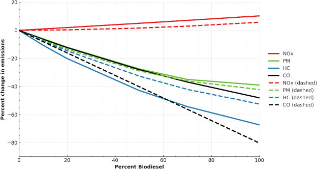
EPA versus Giakoumis (dashed) correlations for the percent change in pollutant emissions of biodiesel blends.
Fontaras et al. [9] measured the effect of B50 and B100 on the Artemis real driving cycle and standard NEDC. The results are depicted against the EPA and Giakoumis correlations to observe the spread (Figs. 2-5). Fontaras et al. stated that when the biodiesel content increases from B50 to B100 during the Artemis real driving cycle, there is a slight increase in PM emissions. In contrast, as biodiesel content increased, NOx emissions decreased for the Artemis and NEDC driving cycles (Fig. 3).
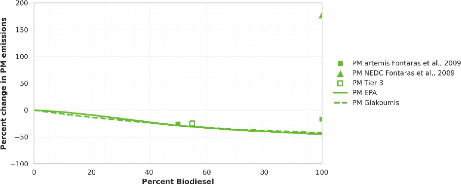
Influence of biodiesel blends on PM emissions.
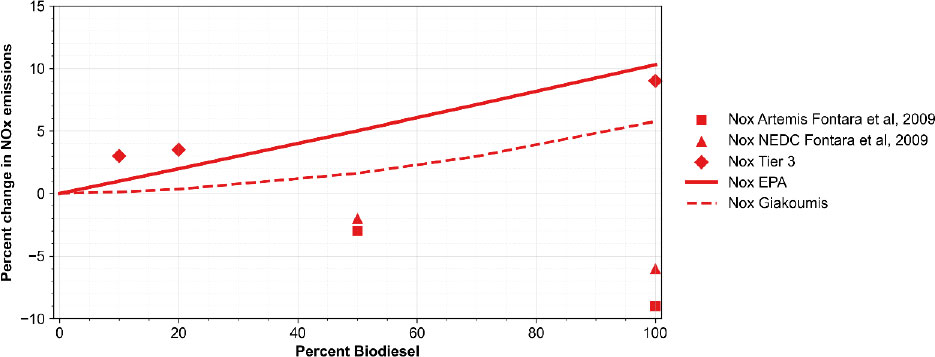
Influence of biodiesel blends on NOx emissions.
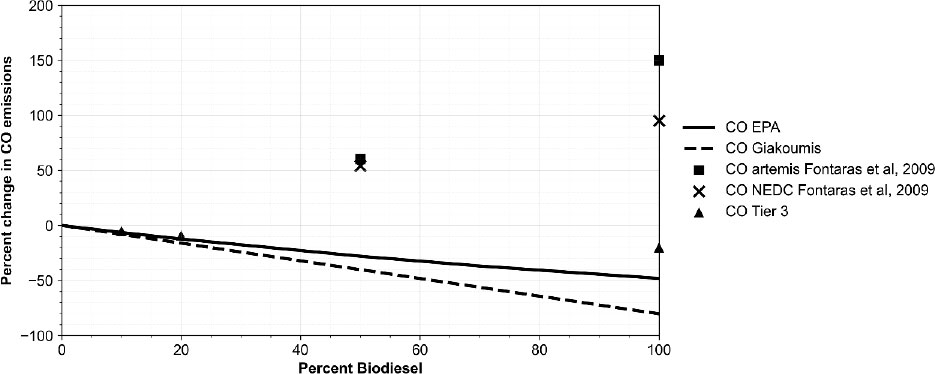
Influence of biodiesel blends on CO emissions.
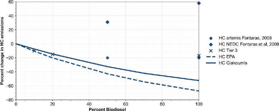
Influence of biodiesel blends on HC emissions.
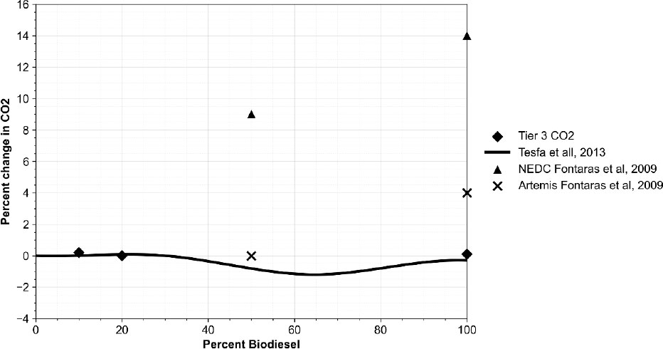
Regarding fuel consumption, an increase was noted, and despite the decrease in carbon content with the addition of biodiesel, the increase in fuel consumption for the same energy generation results in an overall increase (Figs. 6 and 7).
Influence of biodiesel blends on fuel consumption.
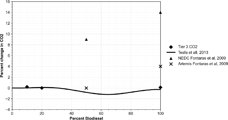
Influence of biodiesel blends on CO2 emissions.
2.2. Tier Approaches
2.2.1. Tier 1 Methodology
The Tier 1 methodology states that emissions are proportional to fuel consumption. This approach is represented by the following formula (Eq. 7):
Ex= Σy (Σm (FCy,m × EFx,y,m)) (7)
Where:
Ex = emission of pollutant x [g],
FCy,m = fuel consumption of vehicle category y using fuel m [kg],
EFx,y,m = fuel consumption-specific emission factor of pollutant x for vehicle category y and fuel m [g/kg]. The emission factors for urban bus standards used in Tier 1 were obtained from a subsequent study [46].
2.2.2. Tier 2 Methodology
This methodology considers the fuel used by different vehicle types and their emission standards. For the application of this methodology, it is important to know the number of vehicles in the fleet, the annual mileage per vehicle, and the Tier 2 emission factors. The algorithm used for the Tier 2 methodology is (Eq. 8):
Ex,y,z = Σy (Ny,z × My,z × EFx,y,z) (8)
Where,
EFx,y,z (grams/kilometer), is the technology-specific emission factor of pollutant x, for vehicle category y and technology z,
My,z (kilometer/vehicle) is the average annual distance driven per vehicle of category y and technology z,
Ny,z is the number of vehicles in a fleet of category y and technology z, respectively.
Vehicles in category y can be classified as passenger cars, light commercial vehicles, heavy-duty vehicles, motorcycles, or mopeds. Each vehicle technology has a specific emission factor, as shown in the study by Ntziachristos et al. [46]. As vehicle technology, one can refer to Euro 1, vehicles introduced in 1992 by Directive 91/441/EEC, being the first with a three-way catalyst; Euro 2, vehicles with better closed-loop, better three-way catalyst control, and lower emission limits compared with Euro 1; and Euro 3, which was introduced in 2000. Vehicles are equipped with lambda sensors to comply with emission limits. Euro 4 was introduced in 2005 with better aftertreatment monitoring and control, and Euro 5 and 6 were proposed by the European Commission in 2007. Euro 5 vehicles have lower NOx emissions than Euro 4.
However, these emission factors are not sensitive to average speed, road slope, or vehicle load. This methodology can capture the effects of A/C, SCR, and biodiesel by applying the correction factor used in the Tier 3 methodology.
2.2.3. Tier 3 Methodology
In the Tier 3 methodology, total emissions are estimated by adding cold to hot emissions; however, the hot emission factors depend on the average circulation speed and type of vehicle. It is important to highlight that Tier 3 does not consider cold emissions from heavy-duty gasoline and diesel vehicles and buses in its analysis, because emission factors are only available for gasoline, diesel, and LPG cars operating as passenger cars or light commercial vehicles. In this manner, only hot emission calculations are detailed in this study. A fundamental factor in this methodology is the average speed of the transportation mode. High emissions are obtained at medium-low speed (Fig. 8A and B); this is related to the stops and starts that the vehicle makes owing to traffic activity.
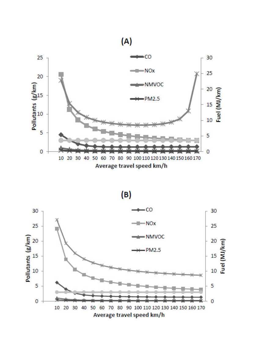
Fuel consumption and pollutant emissions variation with average travel speed for A) Urban Buses Standard 15 t –18 t HD Euro III – 2000 Standards for feeder buses; B) Urban Buses Articulated > 18 t – HD Euro III – 2000 Standards for articulated buses.
Total emissions were calculated by combining the activity data for each vehicle type with the corresponding emission factors. The emission factors vary according to the input data, such as fuel-specific action, fleet activity conditions, driving cycles, and other variables, increasing the uncertainty in the results [46].
Thus, the sensitivity analysis is based on input variations (uncertainty) and observation of output ranges, for example, by using Monte Carlo analysis. A Joint Research Centre report [47] extensively quantified these inputs and the influence of internal variance on the results. For the case studies in the analysis, uncertainty varied with emissions but remained within the 7-44% range, without fuel consumption correction. Nevertheless, these uncertainties do not reflect actual air quality measurements that are cross-checked with emission factors. Therefore, the main question is whether the road transport emission inventory accurately represents the impact of real driving conditions.
In this study, we aim to explore output uncertainty related to different methods, different vehicle load and slope road unknown, lube oil combustion influence unknown, A/C usage and refrigerant leakage influence unknown, biodiesel future blends influence related to its effect uncertainty, extra CO2 emissions due to desulphurization related to its variance, and extra CO2 emissions from refinery desulphurization unit related also to its variance.
2.3. Simulation Scenarios
2.3.1. Characterization of the Case Study
Public transportation in Guayaquil consists of conventional buses, Metrovía (the analyzed BRT system), school buses, and provincial buses. A complete description of the Guayaquil BRT system was obtained through an extensive literature review. The Metrovia BRT system was built in 2006 to control and regulate Guayaquil's urban mass transportation system, seeking efficiency and quality of service. Metrovia buses have exclusive lanes on one-way streets and are diesel-powered with premium diesel of less than 500 ppm sulfur [48]. Table 3 shows detailed information on several indicators for the Metrovia BRT system in 2012, 2014, and 2016.
| Metrovia | Type | km/year | # Buses | Bus Capacity | Operational Speed km/h |
|---|---|---|---|---|---|
| 2012 | Feeders | 77760 | 110 | 90 | 22.8 |
| Articulated | 96120 | 105 | 160 | 25.9 | |
| 2014 | Feeders | 81000 | 200 | 90 | 22.4 |
| Articulated | 99000 | 192 | 160 | 25.6 | |
| 2016 | Feeders | 84960 | 200 | 90 | 22.1 |
| Articulated | 105480 | 205 | 160 | 25.4 |
This data was used because of the availability and consistency of historical databases. In addition, it corresponds to the most recent period for which complete, verified, and comparable data existed, and the other trunk has not yet been completed. Both BRT systems have ‘articulated’ and ‘feeder’ buses with different kilometers per year, passenger capacity, traveled distance, and operational speed. For diesel engine vehicles, such as Metrovia buses, the conventional and HD Euro III – 2000 standards were used as equivalent legislation standards because they comply with the emission limits required for the U.S. 1994 test cycles [49]. All Metrovia buses are equipped with no air conditioning (no A/C), no particle filter (no diesel Particulate Matter Filter (DPF), and no NOx aftertreatment devices (no selective catalytic Reduction-SCR).
The configuration of the fleets can be arranged by structural weight in tons, legislative standard emissions, and fuel type. For our case scenario, two subsectors were applied for the runs: 1) Urban buses standard 15 t – HD Euro III – 2000 standards for feeder buses, and 2) Urban buses articulated > 18 t – HD Euro III – 2000 standards for articulated buses.
The diesel information used in this study was obtained from Petroamazonas records, Technical Report 2673-GCA-REC-12 of the Metropolitan District of Quito, and the requirements set out in the NTE INEN 928 Standard. Information on the purchased diesel fuel in gallons for 2016 was provided by the Metrovia Foundation. The three Metrovia trunks purchased a total of 4.125.077 gallons i13272.90 tons) of diesel fuel in 2016.
The urban bus system in Guayaquil may be changed to improve local air quality by reducing pollutant emissions. This change could involve both technological and fuel improvements. The latter implies at least the construction of a new plant mill. Desulphurizing diesel involves the installation of a desulphurization unit in the refinery by Hydrodesulfurization (HDS) or hydrotreating, which uses a co-feeding oil and H2 in a reactor packed with an efficient inorganic catalyst at high pressure (1–18 MPa) and high temperature (200–450οC). According to the literature, CO2 emissions from the operation range from 5 to 11 g/kgH2 [50–53].
If biodiesel production is considered, the existing endogenous production of the case study must be identified. La Fabril is the only group in Ecuador that produces biodiesel from palm oil and jatropha. This group can potentially process up to 50,000 hectares planted with African palm and jatropha. The actual production in 2016 was 16,259 tons/year, representing 26.6% of its product market share. Its net cultivation productivity is 1 t crude palm oil, which requires 5 t of Fresh Fruit Bunches (FFB) [54, 55]. The transesterification reaction mass flows are as follows: 845 kg of palm oil and 138 kg of anhydrous ethyl alcohol are required to produce 891 kg of biodiesel and 92 kg of glycerin [56]. Given this data, 0.19 hectares are required to produce 1 t of biodiesel, that is, a factor of land use requirements of 0.19 ha/t biodiesel. If this production does not meet the case study needs, additional land will be required to maintain the same production of the other non-energy products, that is, food and cleaning products. This adds 109.62-460.98 kg CO2eq/ t FFB [54] or 520-2186 kg CO2eq/t biodiesel to the overall bioenergy-BRT system.
2.3.2. ‘’What If” Scenarios
Based on actual trends in fuel quality, biofuels, bus Euro emission standards, and exhaust aftertreatment technologies, it is noteworthy to screen what would happen if the Metrovia buses were updated, fitted with A/C and SCR exhaust aftertreatment technology, and fueled with low-sulfur diesel and blended up to 100% biodiesel. Therefore, the COPERT software was implemented. This software is a European emissions inventory model designed to estimate real-world emissions from road transport and evaluate progress toward emission-reduction targets.
For the 2020 air quality, simulations were executed by inserting new emissions standards in the BRT systems, such as Euro IV, Euro V, and Euro VI diesel buses [57]. The Euro V emission standards for trucks were the first control limits that introduced SCR devices to decrease NOx emissions. A backside effect of SCR devices is ammonia (NH3) slippage, which increases emissions at the bus tailpipe. The adoption of the stingiest emission standards was simulated: 50% of the fleet was considered using Euro IV emissions standards, and 100% of the fleet was considered using Euro IV, Euro V, and Euro VI emissions standards. In the Euro V and Euro VI legislation standards, COPERT provides the option to include the percentage share of EGR-equipped vehicles (EGR ratio-%). The SCR ratio (%) was calculated as the 100%-EGR ratio (%). Values for the EGR and SCR ratios were filled in based on market surveys. Different configurations (EGR, SCR, and DPF) were applied to analyze the CO2 emission behavior (Table 4). In the 2012, 2014, and 2016 scenarios, the SCR usage option was not applied due to the old technology still used by BRT buses. Additionally, different biodiesel blends (B0, B10, and B100) and sulfur contents (10 ppm and 450 ppm) were tested. Real-world driving parameters, such as road slopes and vehicle load, were also evaluated in terms of their maximum and minimum influence on the emission results. For instance, the road slope varied between -4% and 4%, and the vehicle load varied between 0 to 100% based on the options that COPERT offers. The normal-based situation implied a 50% vehicle load and 0% road slope.
| Cases | Euro Standard | A/C | UC as a % of FC (%) | SCR/EGR/DPF Usage | |||
|---|---|---|---|---|---|---|---|
| EGR ratio (%) | SCR ratio (%) | DPF (%) | |||||
| Reference | for 2012, 2014 and 2016 | Euro III | NA | NA | 100 | NA | NA |
| “What if” | 1 | Euro III | 100% | NA | 100 | NA | NA |
| 2 | 50% Euro IV 50% Euro III | NA | NA | 100 | NA | NA | |
| 3 | 100% Euro V | NA | 6 | 23.8 | 76.2 | NA | |
| 4 | 6 | 76.2 | 23.8 | NA | |||
| 5 | 6 | 50 | 50 | NA | |||
| 6 | 6 | 0 | 100 | NA | |||
| 7 | 100% Euro VI | 6 | 0 | 100 | 100 | ||
| 8 | 100% Euro VI | 100% | 6 | 0 | 100 | 100 | |
3. RESULTS AND DISCUSSION
The fuel balance provides a control point to compare the statistical fuel consumption provided by the diesel gallons dispatched for Metrovia in 2016 with the total fuel consumption calculated using the Tier 3 methodology. The statistical fuel balance versus Tier 1 and Tier 3 yielded a standard deviation of 26%. This gives an idea of how uncertain the estimates are, 26% for Tier 3 and 39% for Tier 1. This deviation could be produced by several factors related to the actual use of vehicles (e.g., operational speed, traffic conditions, bus capacity and occupation, vehicle load, and road slope). The 26–39% deviation between fuel-balance statistics and Tier 1–3 estimates lies within the 7–44% range reported for European road-transport inventories by Kouridis et al. [47], and is consistent with the spread between laboratory and on-road data for urban buses documented by Zhang et al. [43] and Perdikopoulos et al. [19]. The Tier 3 emission inventory can be used to analyze the influence of such parameters on fuel consumption or emissions. Figure 9 shows that road slopes make a major contribution to the emissions. The inventory of CO2 emissions is uncertain, with a maximum range of -107% to 138% over the average 50% vehicle load and 0% road slope run. The slope and load influence pollutants, such as NOx, which can vary between -50% and 110% over the default conditions of 50% load and 0% slope. These results indicate that the emission inventory is highly sensitive to how vehicle operation is represented, and that relatively small simplifications in the Tier approaches propagate into large uncertainties when applied to a real BRT system.
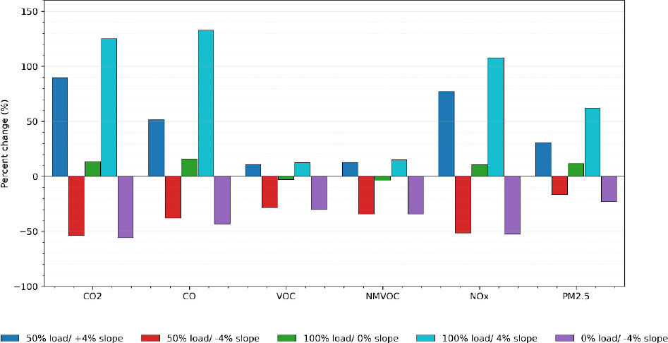
Vehicle load and road slope influence on emissions produced by Metrovia, reference 50% load, 0% slope.
On the other hand, Fig. (10) shows the disaggregation of CO2 emissions by source, either fuel combustion or lube oil combustion, with uncertainty related to which tier methodology is being used.
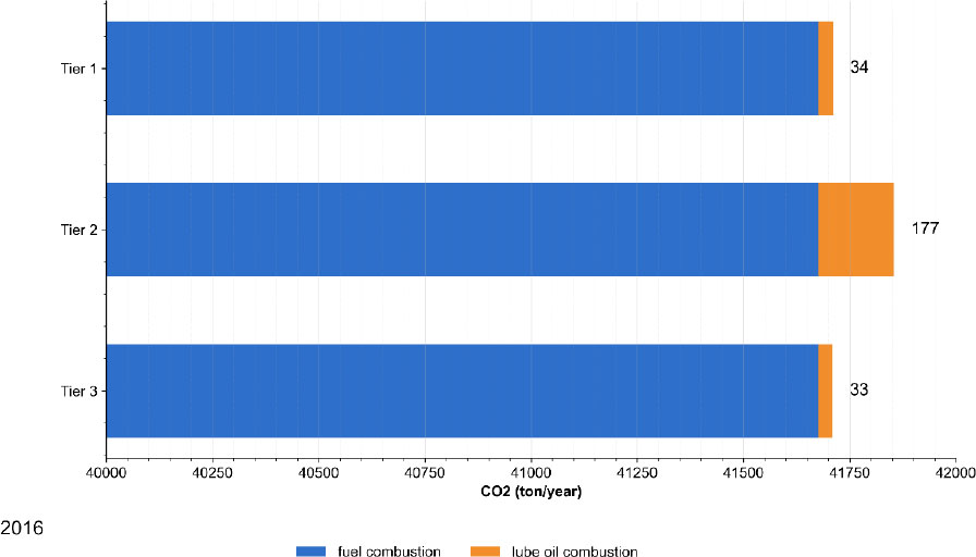
CO2 emissions by source of combustion for Metrovia's case, 50% load, 0% slope.
The uncertainty range in the pollutant emission simulation for the 2016 fleet is shown in Fig. (11). Regardless of the methodology, NOx and CO emissions are supposedly emitted in higher quantities. Our uncertainty analysis revealed that the range of NOx emissions could be very wide, from 433 to 724 tons/year. This range implies that changes in emissions smaller than 40% cannot be distinguished from methodological and operational uncertainty. Consequently, scenarios that yield modest differences should not be used as a basis for stringent regulatory decisions, whereas measures with larger effects remain robust even under the upper uncertainty bounds. The Euro III standards represent another possible method for estimating emissions. The actual values for each emission cannot be determined. Therefore, emissions inventories should include uncertainties that represent the variability of the results across different approaches for their estimation.
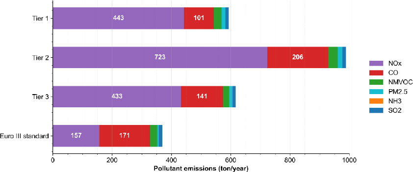
Pollutant emission inventory for 2016. Methodological uncertainty across Tier 1-3 and Euro III approaches (50% load, 0% slope) for 2016.
3.1. ‘’What If” Scenarios
Developing countries tend to keep up with the current trends in Europe or the US. Therefore, it is important to determine the impact on energy consumption and emissions if BRT buses are replaced by buses equipped with A/C, SCR, and DPF, and the fuel quality improves with biofuels entering the market. Both evaluations are based on the maintenance of the number of BRT and activities (i.e., average circulation speed and distance traveled).
If the buses were replaced by Euro VI buses with A/C targeting the comfort of passengers, CO2 emissions would increase due to extra fuel consumption to run the A/C compressor, extra CO2 emissions due to urea SCR, and extra GHG emissions due to A/C leaks. Extra emissions from desulfurization are due to hydrogen production through steam methane reforming. Under real driving conditions, biodiesel could increase CO2 emissions by 14% (Fig. 7). The contribution of each influence to the overall emissions is illustrated in Fig. (12).
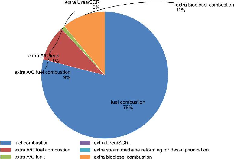
Relative contributions of different CO2 sources for Euro VI fleet equipped with A/C (28°C, 80% humidity) with 10 ppm sulfur and 100% biodiesel.
A/C has the strongest influence on CO2 emissions, mainly due to the extra fuel consumption required to run the compressor. However, passenger comfort is improved and should be implemented to make BRT more attractive. Nevertheless, the contribution of urea is 244 tons of CO2 per year, and the steam methane reforming for hydrogen production and subsequent desulphurization is 12 tons of CO2 per year. The 244 t CO2/year from urea use reflects the stoichiometric CO2 released when urea decomposes in the SCR system. However, the mass of urea consumed is relatively small compared with the mass of fuel burned. As a result, the associated CO2 remains modest in the fleet-wide balance, large enough to be measurable but clearly secondary compared with the fuel penalty of A/C. The 12 t CO2/year attributed to steam methane reforming is small because only a fraction of the refinery’s hydrogen and process energy can be allocated to the diesel volume used by this specific BRT fleet. Even though SMR is a CO2-intensive process, the absolute quantity of fuel demanded by the fleet is limited, so the upstream CO2 burden from desulfurization is also limited in magnitude when expressed on an annual, fleet-only basis. The biodiesel burning influence ranges from 0 to 6,524 tons of CO2 per year. This wide range reflects both the variability in blend levels and the lower Lower-Heating Value (LHV) of biodiesel compared with fossil diesel. Under real driving conditions, the engine must burn more fuel mass per kilometer to deliver the same useful work when the biodiesel content increases. The 20% A/C impact on energy use aligns with Würtz et al. [58], while the relative magnitude of refrigerant leakage and upstream desulfurization CO2 is comparable to the life-cycle contributions reported by Fabris et al. [59].
Pollutant emissions are affected mainly by two sources of change: technological sources, such as air conditioning and selective catalytic reduction urea injection, and fuel-related sources, that is, sulfur reduction and NH3 slip from SCR. Fuel-related changes, that is, biodiesel blends and changing sulfur from 450 to 10 ppm, as well as fitting advanced exhaust aftertreatment, such as selective catalytic reduction and particle filter, have little effect on overall pollutant emissions compared to the air conditioner extra fuel consumption effect (Fig. 13). It is interesting to note that the biodiesel B10 and B100 scenarios are quite similar to B0 owing to the uncertainty range in pollutant emission estimations. This means that within the resolution of the current methodology, switching to B10 or B100 does not produce a statistically separable change in fleet pollutant emissions; any differences are smaller than the inventory’s own noise. The current biodiesel produced by LA Fabril from palm oil, circa 16,259 tons/year, is sufficient to feed the Guayaquil BRT system (13,275 tons, maintaining the current fleet), which means that extra land is not required to cultivate palm trees (0.19 ha/ton biodiesel). However, if this is to escalate to all Ecuadorian cities, there should be a land use change problem and extra CO2 emissions of 520-2,186 kg CO2eq for each ton of biodiesel consumed in addition to the 16,259 tons, as explained in the methodology section. Because of this, biodiesel is sustainable at the current, limited scale in Guayaquil, because it uses existing capacity, but becomes much more carbon-intensive when scaled up, due to the carbon debt associated with expanding palm cultivation.
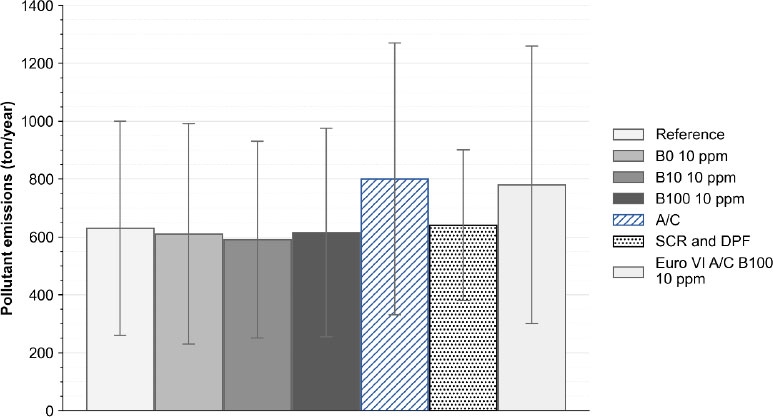
Evolution of pollutant emissions considering fuel “what if” scenarios, technology “what if” scenarios, and both. Results show absolute, fleet-wide annual emissions.
4. LIMITATIONS
This study has several limitations that should be considered when interpreting the results. First, the emission inventories rely on aggregated activity data and fleet statistics for the Guayaquil BRT system; detailed information on duty cycles, instantaneous speeds, passenger loads, and A/C usage was only partially available and had to be represented through simplified profiles. As a result, some operational variability is not fully captured in the Tier 1–3 estimates. Second, the COPERT-based methodology uses default emission factors and correction functions largely derived from European fleets and testing conditions. Although we accounted for these factors to the best of our ability, residual biases may remain for NOx, NH3, and PM, particularly under congested urban operation and for biodiesel blends. Third, the analysis focuses on a specific BRT fleet, refinery configuration, and palm-based biodiesel supply chain; the magnitude of upstream CO2, land-use pressures, and A/C impacts may differ in cities with other fuels, technologies, climates, or topographies. Consequently, our quantitative results should not be generalized directly to all Latin American BRT systems, but rather seen as an illustrative case that highlights the relative importance of A/C, slope/load effects, and upstream fuel pathways under the conditions of Guayaquil.
CONCLUSION
Latin American cities are facing an increase in demand for public transportation systems. For instance, BRT has emerged as a key solution to mobility and environmental concerns. However, accurate quantification of emissions is critical for designing effective mitigation strategies in developing countries. Real-world driving conditions, such as passenger load, road slope, and air-conditioning use, strongly influence the emissions generated by transportation systems. Additionally, fuel changes, such as reducing sulfur ppm and blending diesel with biodiesel, are common measures. The question that emerged in this study was whether bus fuel and technology-related changes would affect energy consumption and emissions. Moreover, it is noteworthy to evaluate the uncertainty using three different tier methodologies. In addition, proposed scenarios were established to analyze what the emissions would be if current buses changed their emission technology, used low-sulfur fuels, mainly biofuels, and if buses used air conditioning systems in the coming years.
Regarding emissions uncertainty and validation of CO2 and SO2 emissions, these are expected to have up to 30%-40% deviation before comparing the fuel estimations with country fuel sales (either Tier 3 or Tier 1 is used). For other pollutants, literature usually claims up to 40% deviation, but this uncertainty should be further investigated. The comparison with fuel statistics and across tiers shows that inventory uncertainties are substantial, but still allow a robust ranking of interventions.
Our uncertainty analysis revealed that the range of NOx emissions could be very wide, from 433 to 724 tons/year. From a policy perspective, the uncertainty bands define a minimum effect size that interventions must exceed to be reliably detected in inventories and air-quality assessments. This threshold is particularly relevant when ranking technology fuel options for BRT renewal. Despite the uncertainty due to the methodology used, some considerations for “what if” scenarios could be made. To improve the Tier 3 methodology for urban buses, auxiliary systems such as air conditioning systems (including leakage), heating systems, and other electrical systems should be included in fuel consumption and emission calculations. Using the same method used for passenger cars (with a correction factor for buses), we found that the A/C influence had a maximum impact of 20% on fuel consumption. This result is similar to that reported by Würtz et al. (2024) [58], who stated that high-voltage air conditioning has the greatest impact on the operational energy consumption of 12 m buses. This is a trade-off risk because, despite increased fuel consumption, the use of A/C on Metrovia buses increases users’ comfort and is more attractive for Guayaquil’s citizens.
Regarding the CO2 emission sources, A/C extra fuel combustion has the highest impact (an extra 20% CO2 emissions from the reference of 46,603 tons/year). A/C refrigerant leakage, urea reaction, and lube oil combustion had a smaller combined impact; nevertheless, they amounted to 863 tons of CO2 per year. Extra CO2 emissions due to the steam reforming reaction amount to 6-12 tons/year. This result is aligned with the findings of Fabris et al. [59]. They found that refrigerant choice and leakage rates can produce substantial CO2-eq contributions at the fleet scale, but are smaller than the A/C fuel effect. Therefore, upgrading the urban BRT fleet and adding thermal comfort to passengers appears to have the greatest impact on fuel consumption, CO2, and pollutant emissions.
Considering the influence of biodiesel, the fuel consumption is expected to increase. Similar results were obtained by He et al. (2024) [60] for a heavy-duty diesel vehicle equipped with a Selective Catalytic Reduction (SCR) system using various palm oil biodiesel-blended fuels. They found that the use of biodiesel blends increased the fuel consumption and affected the pollutant emissions. Variations in pollutant emissions have been reported in the literature. The NOx emissions were inconsistent. In some studies, an increase in another decrease, for example, B50 -3 to +5% and B100 -9% to 10%, was observed. PM2.5 is usually lower, but few studies have reported a 150% increase for B100.
The upstream impacts of biodiesel incorporation into the bioenergy-BRT system should be carefully evaluated because it is feasible for the analyzed case study (Guayaquil), but not for the entire country, without causing upstream issues. For example, to feed the doubled-size BRT fleet, extra land equivalent to roughly 63,000 football fields is required, with an additional GHG emission of 5,350 tons CO2 – 22,490 tons CO2eq. Beyond the methodological uncertainties already discussed, an additional limitation of this study is the restricted system boundary adopted. Although tailpipe emissions and selected upstream CO2 contributions were accounted for, other relevant life-cycle stages remain outside the scope, including the manufacturing, maintenance, and end-of-life phases of buses and infrastructure. As a result, the emission balances presented here should be interpreted as operational and partial upstream impacts of the Metrovia fleet. Even when the upper and lower bounds are considered, the qualitative ranking of interventions is unchanged: A/C remains the dominant additional CO2 source, while changes in pollutant emissions across biodiesel blends are largely masked by inventory uncertainty.
Finally, expensive stationary air-quality monitoring stations are often not feasible in developing countries. Several methodologies for fleet CO, NMVOC, NOx, PM2.5, and NH3 estimates are available. Therefore, Tiers 1, 2, and 3, as well as Euro standards, are used to present the results with uncertainty. To capture the effects (on emissions) of vehicle categories, Euro standards, environmental temperature and humidity, fuel quality, road slope, and vehicle load percentages, Tier 3 should be used. However, Tier 3 should implement updated correlations for biodiesel effects on exhaust emissions and include their uncertainty. Additionally, as a technical recommendation, a small subset of Metrovia buses should be equipped with Portable Emission Measurement Systems (PEMS) or miniaturized exhaust sensors to capture NOx, CO2, NH3 slip, and particulate emissions under real-world driving conditions. Even a campaign covering one or two representative buses per line would allow the calibration of Tier 3 simulations and reduce uncertainty ranges.
AUTHORS’ CONTRIBUTIONS
The authors confirm contribution to the paper as follows: C.M.S.: Study conception and design; D.A.B.: Data collection; C.M.S and D.A.B.: Analysis and interpretation of results; C.M.S., F.C.M., K.E.S. and D.A.B.: Draft manuscript preparation; All authors reviewed the results and approved the final manuscript.
LIST OF ABBREVIATIONS
| BRT | = Bus Rapid Transit |
| IPCC | = Intergovernmental Panel on Climate Change |
| SCR | = Selective Catalytic Reduction |
| NOx | = Nitrogen Oxide |
| EEA | = European Environment Agency |
| CF | = Correction Factor |
| HDV | = Heavy-Duty Vehicle |
| LDV | = Light-Duty Vehicle |
AVAILABILITY OF DATA AND MATERIALS
All the data and supporting information are provided within the article.
FUNDING
The study has been funded by the Instituto Dom Luiz (IDL), under the Project No: UID/GEO/50019/ 2013.
ACKNOWLEDGEMENTS
The authors acknowledge the Instituto Dom Luiz (IDL) for the funding provided. The authors also render their special thanks to Federico von Buchwald de Janon, the Metrovía Foundation, and the INAMHI Institution for providing the data.